From Tokens to Vectors: How Vector Databases Give LLMs Practical Memory

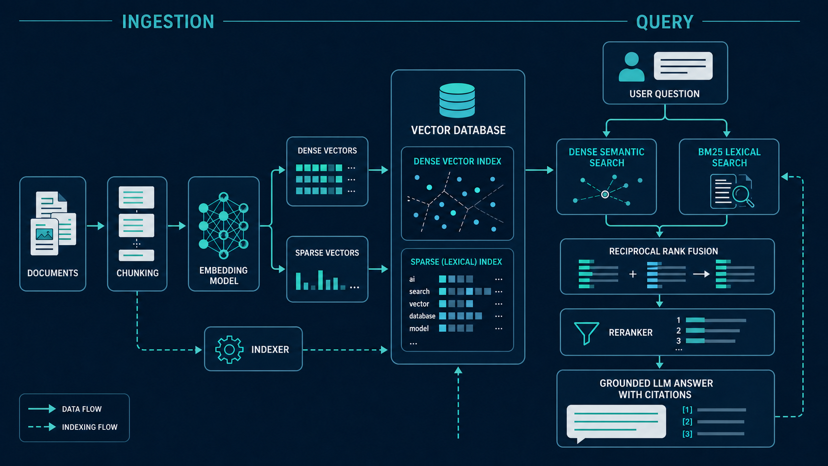
How a production RAG system combines dense retrieval, lexical search, reciprocal rank fusion, and reranking.

Large language models are powerful, but they do not know everything. Their knowledge is learned during training and stored in model parameters. Once training is complete, that knowledge does not automatically change when your product catalog, policies, customer records, or technical documentation changes.

The prompt offers a second source of information, but context windows are finite. Sending an entire document library with every request would be slow, expensive, and often less accurate than sending only the relevant passages.

A vector database solves this retrieval problem. It stores searchable representations of documents outside the model. At query time, the application finds a small set of relevant passages and places them in the prompt. This pattern is commonly called retrieval-augmented generation, or RAG.

The result is not human memory and it is not a permanent extension of the model's brain. It is better understood as dynamic, persistent, non-parametric memory that the application can read and update independently of the model.

In one sentence: A vector database gives an LLM access to current, private, and verifiable knowledge without retraining the model every time the knowledge changes.

What you will learn

By the end of this guide, you will understand how embeddings represent meaning, why hybrid retrieval beats pure semantic search, how HNSW and DiskANN trade memory for speed, and when pgvector is a better choice than a dedicated vector database.

1. The basic architecture

A production RAG system has two major paths.

Ingestion path

1. Collect source data such as web pages, PDFs, tickets, product records, and database rows.

2. Clean and divide the content into useful chunks.

3. Add metadata such as tenant ID, source, document version, language, and access policy.

4. Send each chunk to an embedding model.

5. Store the embedding, source text, metadata, and a stable document identifier.

6. Build a vector index for fast retrieval.

Query path

1. Receive the user's question.

2. Apply authentication, tenant boundaries, and metadata filters.

3. Create an embedding for the query.

4. Run semantic and lexical searches.

5. Fuse and rerank the candidates.

6. Select a small context set.

7. Ask the LLM to answer using that context and cite its sources.

This separation matters. New information can enter through the ingestion path without retraining the LLM. Deleted or restricted information can also be removed from retrieval without changing model weights.

2. The mathematics of meaning

An embedding model maps an input into a point in a high-dimensional vector space:

f(\text{text}) = \mathbf{x}, \quad \mathbf{x} \in \mathbb{R}^{d}

The vector is a list of floating-point values. Similar inputs tend to be placed near each other. For example, "reset a forgotten password" and "recover account access" may be close even though they share few words.

The number of values is the vector's dimensionality. OpenAI's text-embedding-3-small model produces 1,536 dimensions by default. The dimension is part of the storage schema, so changing embedding models requires a migration or a separate vector field.

It is tempting to interpret individual dimensions as named concepts. That is usually incorrect. Meaning is distributed across the full representation. The useful property is the geometry between vectors, not a human-readable label for each coordinate.

Cosine similarity

Cosine similarity compares the direction of two vectors:

\operatorname{similarity}(\mathbf{u}, \mathbf{v}) = \frac{\mathbf{u} \cdot \mathbf{v}} {\lVert \mathbf{u} \rVert\lVert \mathbf{v} \rVert}

A higher value means the vectors point in more similar directions. Cosine similarity is common for text because direction often captures semantic relationship better than raw magnitude.

Euclidean distance

Euclidean distance, also called L2 distance, measures the straight-line distance between two points:

d(\mathbf{u}, \mathbf{v}) = \sqrt{\sum_{i=1}^{d}(u_i-v_i)^2}

A smaller value means the vectors are closer. L2 is useful when absolute geometry matters. Inner product is another common option and can be efficient for normalized embeddings.

The distance function used by the index must match the function used by the query. Teams should validate this choice against real relevance judgments rather than assume one metric is universally best.

3. Parametric and non-parametric memory

An LLM's weights are parametric memory. Fine-tuning changes model behavior by changing those weights. This is useful for tone, formatting, task patterns, or domain behavior. It is usually a poor mechanism for storing facts that change frequently.

A vector store is non-parametric memory. The knowledge lives in records that can be inserted, updated, filtered, audited, or deleted without modifying the model.

The two approaches are complementary. Fine-tune the model for how it should behave. Use retrieval for what it should know right now.

4. Why pure vector search fails

Semantic retrieval is very good at intent. It is less reliable for exact identifiers.

Consider these queries:

• RX-7900-XTX-24G

• INV-2026-004821

• CVE-2026-12345

• Dr. Nadiya Shaikh

An embedding may understand that the first string is a graphics card model, but a semantically similar model number is still the wrong result. The same is true for SKUs, invoice IDs, error codes, email addresses, and proper names.

Lexical search has the opposite strength. BM25 rewards exact or rare term matches and accounts for term frequency, document length, and corpus frequency. It finds identifiers well, but it may miss a passage that expresses the same idea using different words.

Production search should normally use both.

5. Hybrid search with BM25 and dense embeddings

A hybrid retriever runs two searches in parallel:

• Dense retrieval finds semantically similar passages.

• Sparse or BM25 retrieval finds strong lexical matches.

Each retriever returns a ranked list. Their raw scores should not be added directly because cosine and BM25 scores have different scales that can vary by query.

Reciprocal Rank Fusion

Reciprocal Rank Fusion, or RRF, combines result positions instead of raw scores:

\operatorname{RRF}(d) = \sum_{r \in R(d)} \frac{1}{k+r(d)}

Here, r(d) is the position of document d in one ranked list, and k reduces the effect of very small rank differences. A document that ranks well in both lists receives a strong combined score.

RRF is a sensible default when the retrievers use incompatible score ranges. Weighted RRF can help when evaluation data proves that one retriever should matter more for a specific corpus.

Reranking

Fusion produces a candidate set. A reranker then evaluates the query and each candidate more carefully. A cross-encoder or late-interaction model can improve precision because it compares query and document content directly.

The practical sequence is:

1. Retrieve 20 to 100 candidates cheaply.

2. Fuse dense and sparse rankings.

3. Rerank the best candidates with a stronger model.

4. Deduplicate and group chunks by source document.

5. Pass only the best evidence to the LLM.

This keeps cost and latency controlled while improving relevance.

6. Hands-on example with Qdrant

Qdrant can store named dense and sparse vectors on the same point and fuse them in one query. The following example focuses on the retrieval shape. Model names and dimensions should be selected and tested for your corpus.

from qdrant_client import QdrantClient, models

client = QdrantClient(
    url="https://your-cluster.example",
    api_key="YOUR_API_KEY",
    cloud_inference=True,
)

COLLECTION = "support_docs"
DENSE_MODEL = "sentence-transformers/all-minilm-l6-v2"
SPARSE_MODEL = "Qdrant/bm25"

def hybrid_search(query: str, tenant_id: str, limit: int = 8):
    tenant_filter = models.Filter(
        must=[
            models.FieldCondition(
                key="tenant_id",
                match=models.MatchValue(value=tenant_id),
            )
        ]
    )

    return client.query_points(
        collection_name=COLLECTION,
        prefetch=[
            models.Prefetch(
                query=models.Document(text=query, model=DENSE_MODEL),
                using="dense",
                filter=tenant_filter,
                limit=40,
            ),
            models.Prefetch(
                query=models.Document(text=query, model=SPARSE_MODEL),
                using="sparse",
                filter=tenant_filter,
                limit=40,
            ),
        ],
        query=models.FusionQuery(fusion=models.Fusion.RRF),
        with_payload=True,
        limit=limit,
    )

Important production details are easy to miss:

• Apply authorization filters inside retrieval, not after results leave the database.

• Store a stable document_id, chunk_id, and source version.

• Make ingestion idempotent so retries do not create duplicate chunks.

• Keep the embedding model and embedding version in metadata.

• Delete or deactivate old versions when a source changes.

• Treat retrieved text as untrusted input and defend against prompt injection.

• Return source identifiers so the application can show citations.

For teams already operating PostgreSQL, pgvector is a strong alternative. It supports exact search, HNSW, IVFFlat, filtering, sparse vectors, and hybrid retrieval with PostgreSQL full-text search.

7. Exact search and approximate search

Exact nearest-neighbor search compares the query with every eligible vector. Its basic cost grows linearly with the number of vectors:

O(Nd)

For small filtered datasets, exact search can be simple and highly accurate. At millions or billions of vectors, scanning everything for every query becomes too expensive.

Approximate nearest-neighbor indexes reduce the number of comparisons. The trade is that the index may miss a true neighbor. This is why vector search is measured using both speed and recall.

8. HNSW, IVF, PQ, and DiskANN

HNSW

Hierarchical Navigable Small World builds a multi-layer graph. Upper layers provide long jumps across the space. Lower layers refine the search near promising candidates.

HNSW usually provides excellent in-memory latency and a strong recall-to-speed tradeoff. Its main costs are RAM, build time, and slower inserts.

Important controls include:

• M, which controls graph connectivity and memory use.

• ef_construction, which controls build quality and build cost.

• ef_search, which controls query breadth, recall, and latency.

IVF

Inverted File indexing clusters vectors around centroids. A query first finds nearby clusters, then searches only selected lists.

IVF builds faster and uses less memory than HNSW. Its recall depends heavily on cluster quality and the number of lists searched. Searching more lists improves recall but increases latency.

Product Quantization

Product Quantization compresses vectors into short codes. This reduces memory and distance-computation cost. Compression introduces error, so recall can fall. A common design retrieves candidates using compressed vectors and reranks them using full-precision vectors.

DiskANN

DiskANN is designed for collections that do not fit in RAM. It uses a disk-oriented graph, keeps compact Product Quantization codes in memory, and reads selected full vectors from fast SSD storage for more accurate scoring.

DiskANN lowers RAM requirements but adds storage and I/O considerations. Fast NVMe storage is important.

9. Benchmark what users experience

Do not select an index using vendor benchmarks alone. Build a representative evaluation set.

Measure:

• Recall@K: the fraction of known relevant documents present in the first K results.

• NDCG@K or MRR: whether the best results appear near the top.

• p50, p95, and p99 latency: typical and tail response time.

• QPS: sustainable queries per second at the required recall.

• Index build time and ingestion throughput.

• RAM, storage, and network cost.

• Filtered recall under realistic tenant and metadata filters.

• End-to-end answer quality, citation correctness, and abstention behavior.

Multi-tenant filters are especially important. An index may perform well without filters but lose recall when only a small fraction of records belongs to the active tenant.

10. Choosing a vector database

There is no universal winner. The correct choice depends on scale, team skills, consistency requirements, and operational constraints.

Choose pgvector when

• PostgreSQL is already the system of record.

• Transactional consistency and SQL joins matter.

• The current scale fits a well-tuned PostgreSQL deployment.

• The team wants the simplest architecture first.

Choose Qdrant or Milvus when

• Retrieval is a core product capability.

• You need vector-native hybrid search, advanced filtering, or distributed indexing.

• The team can operate another stateful system or use its managed offering.

• Independent scaling of retrieval is valuable.

Choose a managed service when

• Operational simplicity matters more than infrastructure control.

• The team expects rapid growth and wants provider-managed scaling.

• Vendor cost, data location, lock-in, and recovery options have been reviewed.

The safest decision process is to test two candidates using the same corpus, filters, concurrency, and relevance set. Compare total operating cost and answer quality, not only nearest-neighbor latency.

11. A sensible production path

For most teams, the best sequence is simple:

1. Start with PostgreSQL plus pgvector if PostgreSQL already owns the data.

2. Implement hybrid retrieval rather than dense search alone.

3. Create a small golden set of real queries and expected sources.

4. Measure recall, answer quality, tail latency, and filtered behavior.

5. Add reranking only when evaluation shows a clear gain.

6. Move to a dedicated vector system when scale or search features justify the extra operational boundary.

Vector databases do not make an LLM knowledgeable by themselves. They make knowledge retrievable, current, filterable, and auditable. The quality of the final system still depends on chunking, metadata, permissions, fusion, reranking, evaluation, and clear source attribution.

That is the real value of non-parametric memory. It lets a model work with information that can change today without waiting for the model to be trained again.

Sources and further reading

• [OpenAI text-embedding-3-small model documentation](https://developers.openai.com/api/docs/models/text-embedding-3-small)

• [Qdrant hybrid search and reranking](https://qdrant.tech/documentation/advanced-tutorials/reranking-hybrid-search/)

• [Qdrant hybrid query and RRF documentation](https://qdrant.tech/documentation/search/hybrid-queries/)

• [pgvector indexing and hybrid search documentation](https://github.com/pgvector/pgvector)

• [Milvus DiskANN documentation](https://milvus.io/docs/diskann.md)

• [Pinecone indexing overview](https://docs.pinecone.io/guides/index-data/indexing-overview)